1. 损失函数的定义
根据 Y 类型的不同(数值型、类别型、顺序型),一般有三种损失函数:
- Regression loss functions,如 GDP 的预测问题
- Classification loss functions,如区分图片是猫还是狗
- Ranking loss functions,如广告素材的排序问题
本文主要讨论分类问题(classification)的公式推导以及 R
代码示例的实现。
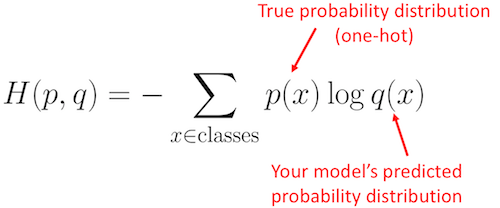
2. 分类问题和交叉熵
交叉熵 Cross entropy loss
是机器学习中常用的衡量分类模型表现如何的指标,熵是由 Claude Shannon 在
1948 年第一次引入。
\[
\begin{equation*}
H(X) = -\Sigma_i P(X=i) \log _2 P(X=i)
\end{equation*}
\]
交叉熵 Cross-entropy
还经常被用于衡量两个概率分布之间的差异。假设有三个类别,标签为
A、B、C,他们的事实分布概率是:
通过训练的某个机器学习分类器,预测的概率分布如下:
我们显然希望预测分布 predicted distribution 同实际分布 true
distribution 无限接近于
0,那这两个分布之间的差异有多大呢?是否在改善?这时候使用的就是交叉熵来度量的,公式如下:
根据公式计算两个分部之间的差异为:
1
2
3
4
5
| d_true <- c(0, 1, 0)
d_predicted <- c(0.228, 0.619, 0.153)
H = -sum(d_true * log(d_predicted))
H
|
目测如果预测改善会出现什么情况:
1
2
3
| d_predicted <- c(0.08, 0.81, 0.11)
-sum(d_true * log(d_predicted))
|
交叉熵变的更小了。假如我们认定预测值大于 0.5 即为 1
的话(传统的分类错误率),会发现这两组的预测精度是一样的(正确率都是
100%),显然无法更好的衡量模型的预测精度。
2.1. 二分类交叉熵
在将问题具象化到二分类问题,交叉熵的损失函数形式为:
\[
\begin{equation*}
L = -(y \log(p) + (1-y) \log (1-p))
\end{equation*}
\]
其中,\(y\) 是真实标签(0 或
1),\(p\) 是模型的预测概率(0 到 1
之间,比如通过 sigmoid 变换的结果)。
通过前面的示例演示以及数学性质,这个损失函数具有两条基本属性:
- 非负性
- 预测目标值越接近实际目标值时,损失函数接越近于 0
2.2. 拟合梯度下降
已知 sigmod 这个变换可以将线性预测的结果压缩到 0 至 1
之间,刚好表征了 0-1 类别的概率
\[
p = \sigma(s)=\frac{1}{1+e^{-s}}=\frac{e}{1+e^{s}}
\]
\(s\) 为 \(x_i\) 的线性组合关系:
\[
s = \sum w_i x_i
\]
我们希望损失函数(交叉熵)最小化,对系数 \(w_i\) 求导:
\[
\frac{\partial L}{\partial w_{i}}=\frac{\partial L}{\partial p}
\frac{\partial p}{\partial s} \frac{\partial s}{\partial w_{i}}
\]
这三项分别计算,可以得到以下结果。推导背景知识可以参考导数推导词条:
\[
\begin{align}
\frac{\partial L}{\partial p} &= -y / p+(1-y) /(1-p) \\
\frac{\partial p}{\partial s} &= e^{s} /\left(1+e^{s}\right) * 1
/\left(1+e^{s}\right)=\sigma(s) *(1-\sigma(s)) \\
\frac{\partial s}{\partial w_{i}} &= x_{i} \\
\end{align}
\]
有了上面推导结果,就可以利用梯度更新的方式求解 \(w_i\):
\[
\begin{equation*}
w_i \leftarrow w_i-\alpha \frac{\partial}{\partial w_i} L(w)
\end{equation*}
\]
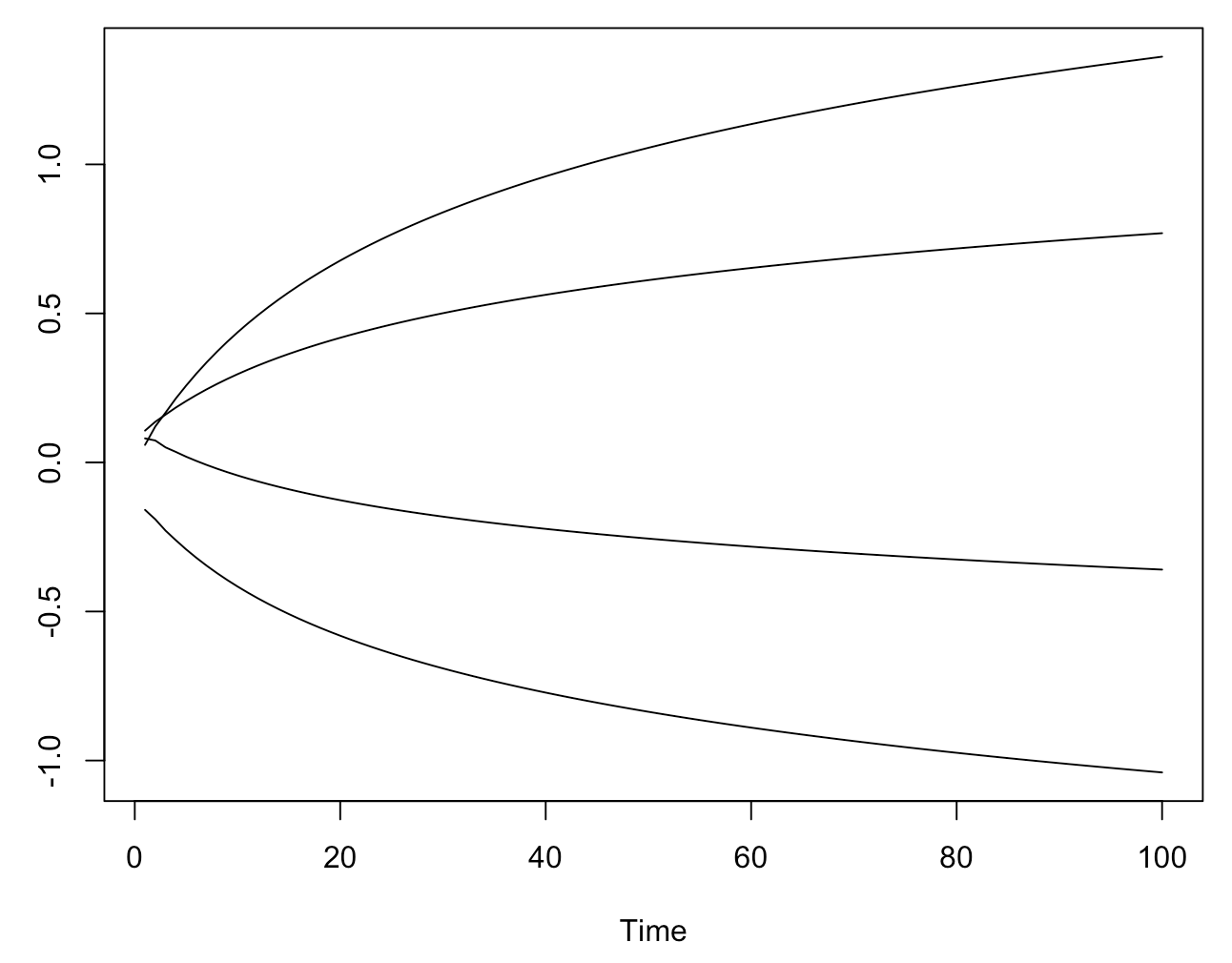
用一个小例子(逻辑回归),来说明 \(w_i\) 更新的过程:
1
2
3
4
5
6
7
8
9
10
11
12
13
14
15
16
17
18
19
20
21
22
23
24
25
26
27
28
29
|
X <- as.matrix(iris[iris$Species != 'versicolor', 1:4])
y <- c(rep(0, 50), rep(1, 50))
nonlin <- function(x, deriv = FALSE) {
if(deriv == TRUE) x * (1 - x)
else 1/(1 + exp(-x))
}
set.seed(1)
w <- rnorm(4, 0, 0.1)
tmp <- list()
for (i in 1:100){
l0 <- X
l1 <- nonlin(l0 %*% w)
l1_delta <- (y - l1) * nonlin(l1, deriv = TRUE)
w <- w + 0.01 * t(l0) %*% l1_delta
tmp[[i]] <- w
}
l1
table(l1 > 0.5, y)
ts.plot(t(do.call(cbind, tmp)))
|
可以观察 coefficient path 的变化:
不过更为通泛的做法是将三者相乘,直接求得 \(\frac{\partial L}{\partial w_{i}}\)
的表达
\[
\begin{align}
\frac{\partial L}{\partial w_{i}} &= [-y / p + (1-y) /(1-p)] *
\sigma(s) *(1-\sigma(s)) * x_{i} \\
&= [-y / \sigma(s)+(1-y)
/(1-\sigma(s))] * \sigma(s) *(1-\sigma(s)) * x_{i} \\
&= [-y * (1-\sigma(s))+(1-y) *
\sigma(s)] * x_{i} \\
&= [\sigma(s)-y] * x_{i}
\end{align}
\]
我们得到了一个比前面推导更加漂亮的结果。将前面的例子重写一下:
1
2
3
4
5
6
7
8
9
10
11
12
13
14
15
16
17
18
19
20
21
22
23
|
X <- as.matrix(iris[iris$Species != 'versicolor', 1:4])
y <- c(rep(0, 50), rep(1, 50))
sigmoid <- function(x){
1/(1 + exp(-x))
}
w <- rnorm(4, 0, 0.1)
tmp <- list()
for (i in 1:100){
l0 <- X
l1 <- sigmoid(l0 %*% w)
w <- w + 0.001 * t(l0) %*% (y - l1)
tmp[[i]] <- w
}
l1
table(l1 > 0.5, y)
ts.plot(t(do.call(cbind, tmp)))
|
3. 为什么不用 MSE
从前文可以看到,交叉熵权重学习的速率受到 \(\sigma(s) - y\)
的影响,也就是输出误差的控制,这样在误差较大时有更大的学习速度。再比较一下平方损失代价函数的学习速率,定义
Loss 为:
\[
L=\frac{1}{2}\left(p-y)^{2}\right.
\]
且
\[
p = \sigma(s)=\frac{1}{1+e^{-s}}=\frac{e^{s}}{1+e^{s}}
\]
则对其求偏导有
\[
(p-y) * \sigma(s) *(1-\sigma(s)) * x_{i}
\]
不难看出,其偏导值在输出概率值接近0或者1的时候都会非常小,这可能会造成模型刚开始训练时,偏导值几乎消失。
这也是为什么我们不会使用 MSE 作为 0-1 回归 loss 的原因。
4. 标准神经网络
构建包含一个隐藏层 hidden layer 的神经网络,隐藏层有两个 cell。
1
2
3
4
5
6
7
8
9
10
11
| library(visNetwork)
color.background <- c("red","red","red","red","blue","blue","green")
nodes <- data.frame(id = c(1,2,3,4,5,6,7),
color.background = color.background,
label = c('I1', 'I2', 'I3', 'I4', 'H1', 'H2', 'O1'))
edges <- data.frame(from = c(1,2,3,4,1,2,3,4,5,6),
to = c(5,5,5,5,6,6,6,6,7,7),
label = c(rep('', 10)))
visNetwork(nodes, edges, width = "100%") |>
visEdges(arrows = "to") |>
visHierarchicalLayout(sortMethod = 'directed')
|
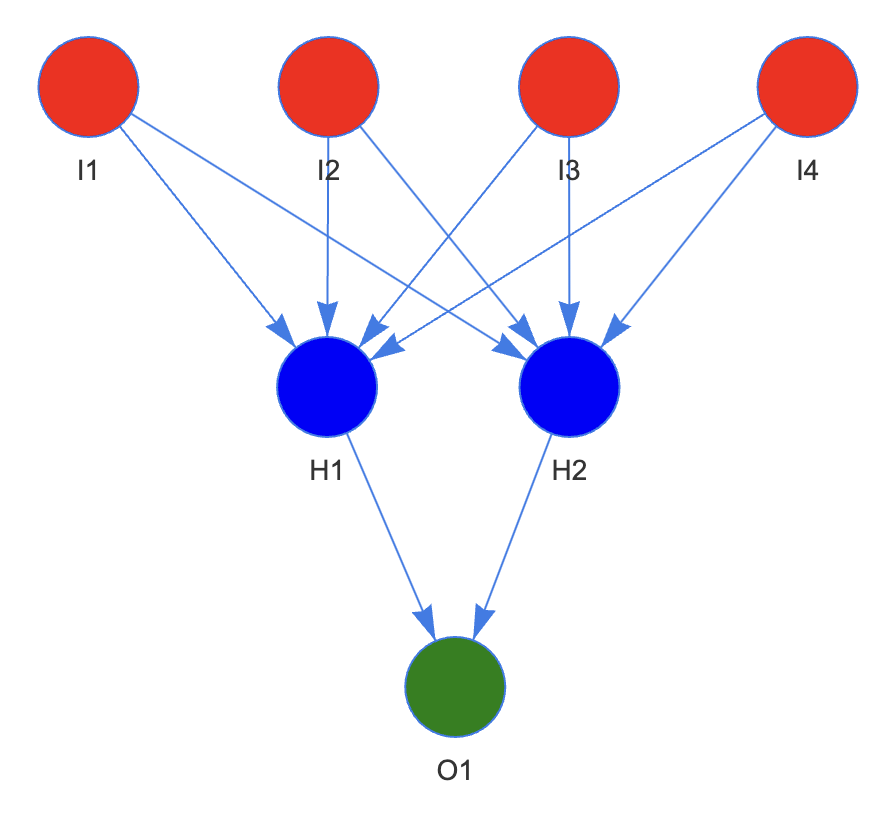
看看每个层的参数是如何更新的,两个关键映射
- 4 个变量向 2 个 cell 的 sigmoid 映射
- 2 个 cell 向 y 的 sigmoid 映射
对应的代码如下:
1
2
3
4
5
6
7
8
9
10
11
12
13
14
15
16
17
18
19
20
21
22
23
24
25
26
27
28
29
30
31
32
33
34
35
36
37
38
39
40
41
|
X <- as.matrix(iris[iris$Species != 'versicolor', 1:4])
y <- c(rep(0, 50), rep(1, 50))
nonlin <- function(x, deriv = FALSE) {
if(deriv == TRUE) x * (1 - x)
else 1/(1 + exp(-x))
}
set.seed(1)
m <- ncol(X)
n <- 2
syn0 = matrix(rnorm(m*n, 0, 0.1), nrow = m, ncol = n)
syn1 = rnorm(n, 0, 0.1)
iter <- 500
M <- matrix(0, iter * 3, 3)
M[,1] <- rep(1:iter, 3)
M[,3] <- rep(1:3, each = iter)
for(j in 1:iter){
l0 <- X
l1 <- nonlin(l0 %*% syn0)
l2 <- nonlin(l1 %*% syn1)
l2_delta = (y - l2) * nonlin(l2, deriv = TRUE)
l1_error = l2_delta %*% t(syn1)
l1_delta = l1_error * nonlin(l1, deriv = TRUE)
syn1 <- syn1 + 0.01 * t(l1) %*% l2_delta
syn0 <- syn0 + 0.01 * t(l0) %*% l1_delta
M[j,2] <- sd(y - l2)
}
pred <- X %*% syn0 %*% syn1 |> nonlin()
table(pred > 0.5, y)
|
能不能加快迭代速度?显然是可能的,有两个思路:
- 标准化
- 中心化
我们看看这两个思路的效果如何?
1
2
3
4
5
6
7
8
9
10
11
12
13
14
15
16
17
18
19
20
21
22
23
24
25
26
27
28
29
30
31
32
33
34
35
36
37
38
39
40
41
42
43
| m <- ncol(X)
n <- 2
syn0 = matrix(rnorm(m*n, 0, 0.1), nrow = m, ncol = n)
syn1 = rnorm(n, 0, 0.1)
for(j in 1:iter){
l0 <- scale(X)
l1 <- nonlin(l0 %*% syn0)
l2 <- nonlin(l1 %*% syn1)
l2_delta = (y - l2) * nonlin(l2, deriv = TRUE)
l1_error = l2_delta %*% t(syn1)
l1_delta = l1_error * nonlin(l1, deriv = TRUE)
syn1 <- syn1 + 0.01 * t(l1) %*% l2_delta
syn0 <- syn0 + 0.01 * t(l0) %*% l1_delta
M[j + iter,2] <- sd(y - l2)
}
m <- ncol(X)
n <- 2
syn0 = matrix(rnorm(m*n, 0, 0.1), nrow = m, ncol = n)
syn1 = rnorm(n, 0, 0.1)
for(j in 1:iter){
l0 <- t(t(X) - colMeans(X))
l1 <- nonlin(l0 %*% syn0)
l2 <- nonlin(l1 %*% syn1)
l2_delta = (y - l2) * nonlin(l2, deriv = TRUE)
l1_error = l2_delta %*% t(syn1)
l1_delta = l1_error * nonlin(l1, deriv = TRUE)
syn1 <- syn1 + 0.01 * t(l1) %*% l2_delta
syn0 <- syn0 + 0.01 * t(l0) %*% l1_delta
M[j + 2*iter,2] <- sd(y - l2)
}
M <- data.frame(M)
M <- transform(M, X3 = as.factor(X3))
names(M) <- c('iter','MSE','Class')
library(ggplot2)
ggplot(data = M, mapping = aes(x = iter, y = MSE, colour = Class)) +
geom_line(linewidth = 1.5) + ylim(0,.65)
|
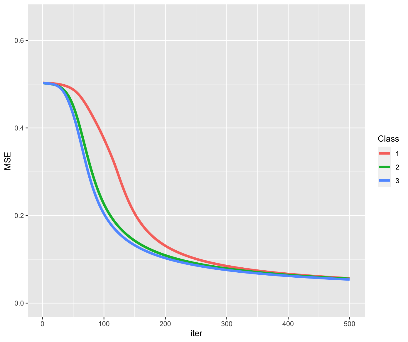
可以看到标准化和中心化都可以更快速的求得结果。